DESeq2做差异基因分析

November 06, 2022 RNASeq 阅读量：次

值得好好读一下：

https://hbctraining.github.io/DGE_workshop/lessons/04_DGE_DESeq2_analysis.html

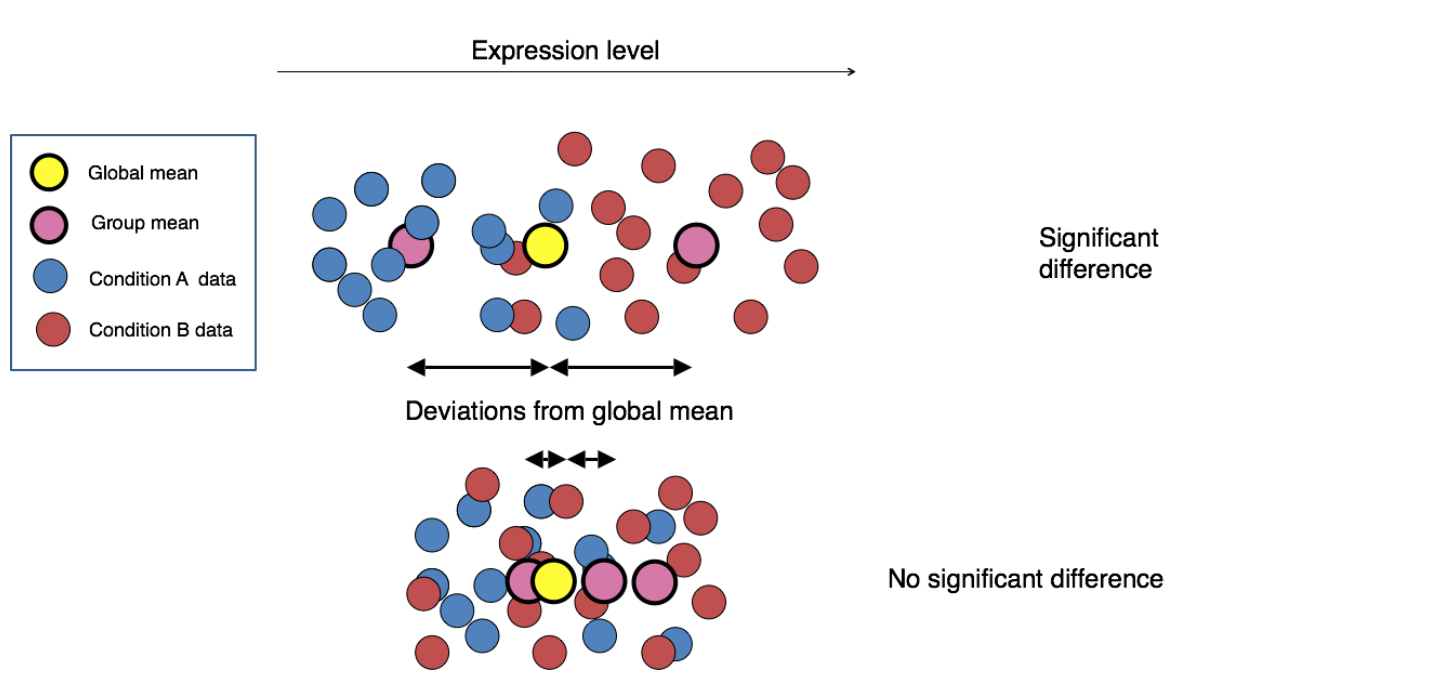
对于组学分析来说，常常会寻找组间的差异，例如差异基因（转录组）、差异菌（宏基因组）以及差异通路（宏基因组），而转录组分析上最为经典的DESeq2包对于以上分析也都适用

DESeq最早在2010年发表在Genome Biology上，2014年上更新版本DESeq2。DESeq2是基于负二项广义线性模型估算样本间基因差异表达概率，既适于有生物学重复的也适于没有生物学重复的样本，同时除了在转录组学，在宏基因组上使用DESeq2计算差异菌的也有报道

一、1.基本原理

1.1 概述

全称：DESeq2 package for differential analysis of count data;
利用负二项分布广义线性模型( negative binomial generalized linear models），同时，还利用了离散型估计、logFoldChange;
负二项分布是一个离散分布，符合测序reads分布；

1.2 构建dds

要求输入原始 reads count 数；不接受已经做过处理的FPKM/TPM等，因为软件有自己的标准化计算方法；
构建dds。需要设置design公式，即告诉软件你的数据是怎样来的，基本试验设计如何，软件会根据几个变量综合计算；

一般：design =~ variable1 + variable2 + …；只有一个变量时：design=~ condition；很多医学分析会加入年龄、性别等：design=~sex+disease+condition；可以对应几个变量，但如果没有额外参数，log2FC和p值是默认对design公式中的最后一个变量或者最后一个因子与参考因子进行比较；

1.3 函数与计算

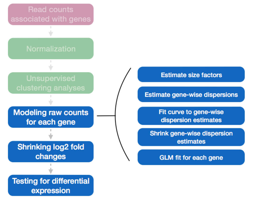
1.3.1 标准化：DESeq函数

不同样品的测序量有差异，最简单的标准化方式是计算counts per million (CPM) = 原始reads count ÷ 总reads数 x 1,000,000；
这种计算方式，易受到极高表达且在不同样品中存在差异表达的基因的影响：这些基因的打开或关闭会影响到细胞中总的分子数目，可能导致这些基因标准化之后就不存在表达差异了，而原本没有差异的基因标准化之后却有差异了；
RPKM、FPKM、TPM 是 CPM按照基因或转录本长度归一化后的表达，都会受到这一影响；

DESeq2的方法：

量化因子 (size factor,SF)，首先计算每个基因在所有样品中表达的几何平均值；每个细胞的SF是所有基因与其在所有样品中的表达值的几何平均值的比值的中位数；由于几何平均值的使用，只有在所有样品中表达都不为0的基因才能用来计算。这一方法又被称为RLE(relative log expression)。
不但考虑了测序深度的问题，还考虑了表达量超高或者极显著差异表达的基因导致count的分布出现偏倚。

DESeq函数分析：

三步：estimation of size factors（estimateSizeFactors)， estimation of dispersion（estimateDispersons)， Negative Binomial GLM fitting and Wald statistics（nbinomWaldTest）；
可以分步运行，也可一步到位，最后返回 results可用的DESeqDataSet对象。

1.3.2 归一化：rlog/vst

我用在对dds进行vst然后做PCA分析。

全称：快速估算离散趋势并应用方差稳定转换；

若 samples<30 用 rlog函数，>30用 vst；

类似的函数：gmodels - fast.prcomp，输入数据为TPM；或者TMM；

1.3.3 数据收缩：lfcShrink：

shrink the log2 foldchange，不会改变显著差异的基因总数，作者很推荐这个新功能。

为何采用lfcShrink？log2FC estimates do not account for the large dispersion we observe with low read counts. 因此，两种数据特别需要：低表达量占比高的；数据特别分散的。
说的就是我的数据啊！但是我只用来做MA plot并没用来差异分析，因为：
lfcShrink 不改变p值q值，但改变了fc，使 foldchange范围变小，所以选择DEG时会有不同结果，一般会偏少！所以，根据数据情况，本次分析DEG还是不做shrink。

1.3.4 p-value和q-value

作者给出的建议：

Need to filter on adjusted p-values, not p-values, to obtain FDR control. 10% FDR is common because RNA-seq experiments are often exploratory and having 90% true positives in the gene set is ok. 即：用padj为标准做结果筛选。

事实上，在软件计算过程中，多次以alpha表示padj，并默认alpha=0.1；

1.3.5 MA plot

MA plot也叫 mean-difference plot或者Bland-Altman plot，用来估计模型中系数的分布;
X轴, the “A”(average)；Y轴，the “M”(minus) – subtraction of log values is equivalent to the log of the ratio;
M表示log fold change，衡量基因表达量变化，上调还是下调；A表示每个基因的count的均值；根据summary(res)可知，low count的比率很高，所以大部分基因表达量不高，也就是集中在0的附近（log2(1)=0，也就是变化1倍），提供了模型预测系数的分布总览。
本次做了lfcshrink+batch之后，MA图趋于正常，比较集中在0附近，一些差异基因也可以明显看出。

1.4 DESeq(dds)结果矩阵每一列的含义：

baseMean： is a just the average of the normalized count values, dividing by size factors, taken over all samples in the DESeqDataSet；是对照组的样本标准化counts的均值；
log2FoldChange： the effect size estimate. It tells us how much the gene’s expression seems to have changed due to treatment with dexamethasone in comparison to untreated samples；也不是简单的用标准化的counts进行计算，因为计算的时候需要考虑零值以及其他效应；结果是log2fc(trt/untrt)所以要注意对照和处理的指定；
lfcSE： the standard error estimate for the log2 fold change estimate，(the effect size estimate has an uncertainty associated with it,)；
p value: statistical test , the result of this test is reported as a p value. Remember that a p value indicates the probability that a fold change as strong as the observed one, or even stronger, would be seen under the situation described by the null hypothesis；
p value有时候是NA：Sometimes a subset of the p values in res will be NA (not available); This is DESeq’s way of reporting that all counts for this gene were zero, and hence no test was applied. In addition, p values can be assigned NA if the gene was excluded from analysis because it contained an extreme count outlier. For more information, see the outlier detection section of the DESeq2 vignette.
padj: adjusted p-value;

1.5 实际遇到的其它问题

1.5.1 pre-analysis 预分析

就是开始熟悉你的数据，知道ta的特点，ta是什么样子什么脾气秉性，什么方式更能发现真实的ta，什么方式能扬长避短！选择合适的分析方法；

先做PCA！方法包括且不仅包括：

gmodels - fast.prcomp
DESeq2 - vst - plotPCA

1.5.2 批次效应

1.本项目的批次效应：

根据预先进行的PCA和correlation结果，本项目样品individual间的差异性大于不同处理的差异；
若不去除，则根据不同A处理寻找DEG时必然会因为individual的影响而覆盖掉一些，导致结果偏少；（test事实证明确是如此）；（本项目也做了removebatchEffect但是仅仅为了展示和验证）；
因此，将4个体当做4个批次，写入design公式： design =~ individual + condition

2.一般批次效应：

可以用limma removeBatchEffect或者Combat等去除；
但是在做差异分析时，ballgown, DESeq2等软件建议不要提前去批次，而是将批次作为covariate进行分析。

1.5.3 多组比较

若有好几组处理，想两两比较，是分开准备数据、DESeq、results？还是全部数据一起？（注意：是几组之间两两比较，不是一比多，一比多请移步多重t检验或者WGCNA，作者Mike Love也说不能做！）

官方建议：

如有多个组需要比较，建议不要将其两两分开而是一起分析，通过在results时指定contrast对象，获得两两的比较结果，这样可以综合考虑所以样品中的表达计算量化因子做DESeq；
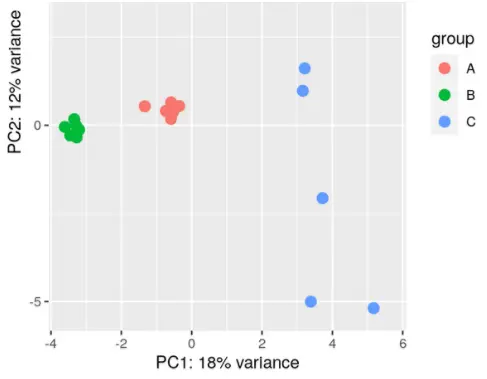
但是，如果你通过PCA/EDA分析发现某一组或某几组的within-group variability比其他组的大，那么还是还是两两分组分开比较吧！

举例，下面的情况就不适合一起做：（这可不就是我的数据嘛！所以，分开比较分别做DESeq更sensitive。）

1.5.4 低表达量基因过滤

1.实际分析完后，我发现一些假阳性DEG，即由于一个样本中出现极高reads而其它样本都是0 reads导致的DEG，在bioconductor上发帖得到了作者回复，于是加入附加条件：筛除在少于3个样品中表达量少于10 reads的基因，再做DESeq标准化和DEG筛选。

2.举例：有一个基因仅仅因为在处理2中有一个表达而其他都是0，就被认为是处理2/1的上调和处理3/2的下调，很不靠谱；

解决：（这个标准可以根据数据特点，自己制定）

keep <- rowSums(counts(dds) >= 10) >= 3   
dds <- dds[keep, ]

1.5.5 outliers离群值处理

这部分提前写了，outliers是在results之后，summary(res)可以看到差异比较的一个基本结果，有一项outliers，若占比很高数量成百上千，则要引起警惕。解决方法：

软件作者提到：

The automatic outlier filtering/replacement is most useful in situations which the number of outliers is limited. When there are thousands of reported outliers, it might make more sense to turn off the outlier filtering/replacement (DESeq with minReplicatesForReplace=Inf and results with cooksCutoff=FALSE) and perform manual inspection.

就是说离群值太多的话还是关闭这一筛选功能，方法也提到了：

minReplicatesForReplace = Inf 
results with cooksCutoff = FALSE

实践证明两个条件择一即可，outliers消失，很多假阴性降低。

分析前可以做一个欧氏距离计算，看是不是有样本特别高或者低，可以剔除，方法见脚本。

二、前期准备

2.1 安装并导入DESeq2包

判断是否有BiocManager包，若不存在则安装

options(repos=structure(c(CRAN="https://mirrors.tuna.tsinghua.edu.cn/CRAN/"))) #设置清华镜像，加速下载

if (!requireNamespace("BiocManager", quietly = TRUE))
install.packages("BiocManager")
if (!requireNamespace("DESeq2", quietly = TRUE))
BiocManager::install('DESeq2')  #通过BiocManager安装DESeq2 
library(DESeq2) #加载library

2.2 数据准备

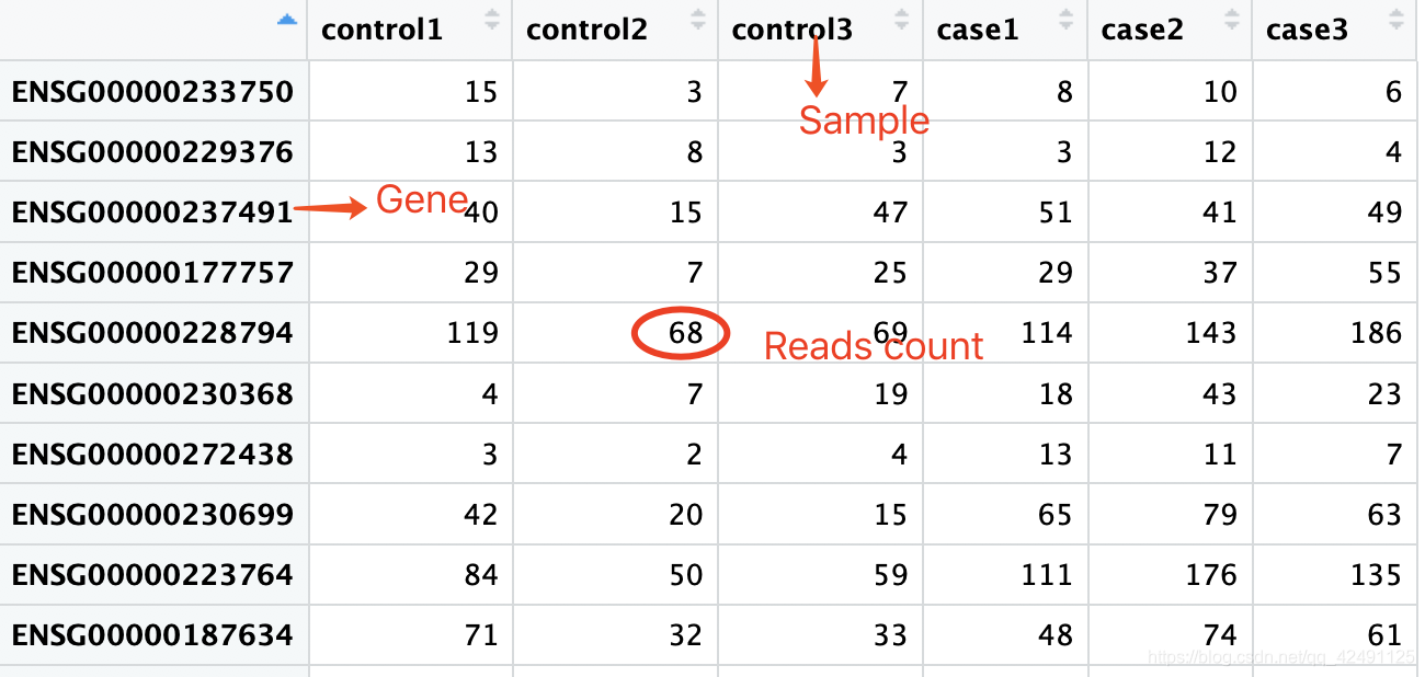
1.基因表达矩阵countData

行为基因，列为样本，需要注意表达数据为原始reads count，DESeq2内部会根据样本大小对counts进行调整，自带标准化过程，不要使用标准化后的FPKM或TPM

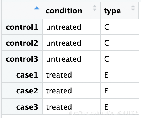
2.样本分组信息 colData

样品信息，第一列是样品名称，第二列是样品的处理情况（对照还是处理等），即condition，condition的类型是一个factor，第三列可添加其他信息（可选）。需要自己根据临床/实验分组信息单独建立

3.制作dds对象，进行差异分析

想要进行差异分析，首先需要生成DESeq2必须的数据类型，即dds类型数据，DESeq2包使用DESeqDataSet(dds)作为存放count数据及分析结果的对象，每个DESeqDataSet(dds)对象都必须由以下三者：

countData ，存放counts matrix的对象
colData ，存放分组信息和处理信息的对象
design公式，对应sample的分组信息，需要以~ 波浪字符进行连接，而不同的信息之间需要以+连接，示例:design=~variable_1 + variable_2

这些分组信息会被用来估算离散度和估算Log2 fold change的模型注意，为了方便起见，在默认参数下，用户应该把感兴趣的分组信息放在formula的最后，并且确认control组的level是第一个

代码如下：

getwd()  #显示当前工作目录
setwd()  #设置工作目录

#install.packages("readxl")
library(readxl)

setwd("D:/project/cancer/IL12/1.analysis/biomarker/")

> database<-read_excel("D:/project/cancer/IL12/0.ref/转化医学/IL-12 IIT Oncomine RNA analysis 20230912 update.xlsx",sheet = "reads" )

> row.names(database) = database$Gene
Warning message:
Setting row names on a tibble is deprecated. 
> database = data.frame(database[,-1],row.names = rownames(database))

> head(database)
         W154012001T2 W154012005T2 W154012009T2 W154012011T2 W154012012T2
PTPRCAP             6           67           38            0           27
KIR2DL2             0            0            0            0            1
CTAG2            1827            0            0           36           22
CX3CR1_1           31           52           59            0           17
CX3CR1_2            0            0            0            0            3
CX3CR1_3            4            0            0            0            0
         W154012013T2 W154012014T2 W154012015T2 W154012016T2 W154012019T2
PTPRCAP             0           64            5           20           22
KIR2DL2             0            0            0            0            0
CTAG2               0            0            0            0            1
CX3CR1_1          379           73          183           85          593
CX3CR1_2            0            1            6            1            5
CX3CR1_3            0            0            2            1           29
         W154012024T2 W154012029T2 W154012030T2 W154012045T2 W154012046T2
PTPRCAP            17           14           18           11           13
KIR2DL2             0            0            0            0            0
CTAG2               0            7           15            0            0
CX3CR1_1           44          135           82           93           56
CX3CR1_2            2            2            0            5           32
CX3CR1_3            3            3            0            0            4
         W154012051T2 W154012052T2 W154012061T2 W154012062T2 W154012063T2
PTPRCAP            27            2            0           12           37
KIR2DL2             0            0            0            0            0
CTAG2               0            0           61        11384         8634
CX3CR1_1            0           32          134           29           36
CX3CR1_2            0            2            0            0            0
CX3CR1_3            0            0            0            0            0
         W154012064T2 W154012065T2 W154012066T2 W154012067T2 W154012068T2
PTPRCAP            20           20           57            0            2
KIR2DL2             0            0            0            0            0
CTAG2               0            0            0            0            0
CX3CR1_1          349          163          257          134           58
CX3CR1_2            0            2            2            0            0
CX3CR1_3           10            0            0            0            7

##coldata

coldata<-read_excel("D:/project/cancer/IL12/0.ref/转化医学/IL-12 IIT Oncomine RNA analysis 20230912 update.xlsx",sheet = "condition" )

#coldata <- subset(coldata,duplicated(sampleid) | duplicated(sampleid, fromLast=TRUE))
#database <- database[,coldata$sample]  # 提取相关的18列

sorted_col <- coldata[order(match(coldata$sample, colnames(database))), ]

row.names(sorted_col) = sorted_col$sample

sorted_col = data.frame(sorted_col[,-1],row.names = rownames(sorted_col))

###dds

dds <- DESeqDataSetFromMatrix(countData = database, colData = coldata, design = ~ condition);

dds

解释：

estimating size factors：估算库size factor
estimating dispersions：估算离散度
gene-wise dispersion estimates：估算基因的离散度
mean-dispersion relationship：均值-离散度关系
final dispersion estimates：估算最终离散度
fitting model and testing：模型适应和测试

指定比较组

默认情况下，R语言根据字母顺序为因子指定水平。如果未告诉DESeq2与哪个水平进行比较（例如，对照组），则基于字母顺序经行比较。

有两种指定比较组的方法：

#方法1： 指定因子水平（要求对照组在前）
dds$condition <- factor(dds$condition, levels = c("untreated","treated"))

#方法2或者直接指定对照组(对照组在前)，此种方法更直观一点；
dds$condition <- relevel(dds$condition, ref ="untreated")
dds$condition

我的案例：

sorted_col <- coldata[order(match(coldata$sample, colnames(database))), ]

row.names(sorted_col) = sorted_col$sample

sorted_col = data.frame(sorted_col[,-1],row.names = rownames(sorted_col))


# dds_norm$condition   #保证是levels是按照后一个比前一个即trt/untrt，否则需在results时指定
# Levels: Post Pre  我这明显是反了的

dds$condition <- relevel(dds$condition, ref = "Pre")  # 指定比較的
dds$condition
# Levels: Pre Post


dds$condition <- relevel(dds$condition, ref = "Pre")  # 指定比較的
dds$condition

4. PCA分析

keep <- rowSums(counts(dds) >= 10) >= 3   #过滤低表达基因，至少在3个样品中都有10个reads 
dds <- dds[keep, ] 

vsdata <- vst(dds, blind=FALSE)  #归一化
assay(vsdata) <- limma::removeBatchEffect(assay(vsdata), vsdata$individual)  #去批次效应
plotPCA(vsdata, intgroup = "condition") #自带函数

三、分析流程

筛选差异基因:

一般按照pvalue < 0.05 & |log2FoldChange| >1筛选差异基因，如果想要结果更可靠，可选择使用更严谨的padj和更大的log2FoldChange进行筛选最后可分别保存差异上调和差异下调的基因：

filter_up <- subset(res, pvalue < 0.05 & log2FoldChange > 1) #过滤上调基因
filter_down <- subset(res, pvalue < 0.05 & log2FoldChange < -1) #过滤下调基因

得到差异基因之后，可进行基因功能富集、PCA和热图聚类等后续分析

3.1 差异分析结果

dds <- DESeq(dds)	#正式进行差异分析

#dds_norm <- DESeq(dds, minReplicatesForReplace = Inf) #标准化; 不剔除outliers; 与cookscutoff结果相同
#dds_norm$condition   #保证是levels是按照后一个比前一个即trt/untrt，否则需在results时指定
# res <- results(dds_norm, contrast = c("condition","treat2","treat1"), cooksCutoff = FALSE) #alpha=0.05可指定padj; cookCutoff是不筛选outliers因为太多了

判断欧氏距离，若有异常样品则不用cooksCutoff；当有上千个异常值时也不用：（完全可以不做）

par(mar=c(8,5,2,2))
boxplot(log10(assays(dds_norm)[["cooks"]]), range=0, las=2)

#使用results()函数提取分析结果； #treated vs untreated表示log2(treated/untreated)，untreated为对照；

#使用生成结果指定比较组的两种方法：
res <- results(dds, contrast=c("condition","treated","untreated"))
#name:the name of the individual effect (coefficient) 用于连续型变量；
#res <- results(dds, name="condition_treated_vs_untreated")
#也可改变顺序（引起log2FC列正负号变化而已）；
res <- results(dds, contrast=c("condition","untreated","treated"))
#如果是多个分组，如何指定特定几个比较组？
# results(dds, contrast=c("condition","treated1","untreated"))
# results(dds, contrast=c("condition","treated2","untreated"))

关于并行运算。DESeq()函数的运算耗时一般小于30s，results()函数提取现成结果非常快可不用并行运算。执行并行运算的方法一是使用DESeq()中parallel= TRUE，BPPARAM=MulticoreParam(4)两个参数；方法二是在分析前注册4个核心，然后DESeq()函数就可以并行运算了，这里设置4个核心。

#并行运算；
#library("BiocParallel")
#register(MulticoreParam(4))
#dds <- DESeq(dds，parallel = TRUE)

#关于p-values和adjusted p-values；
#根据p value，堆结果进行升序排列:
resOrdered <- res[order(res$pvalue),]
resOrdered

##提取结果，在treated和 untreated 组进行比较

res <- results(dds, contrast = c("condition", "treated", "untreated"))

#results从DESeq分析中提取出一个结果表，从而给出样品的基本均值，log2倍变化，标准误差，测试统计量，p值和校整后的p值；

resordered <- res[order(res$padj),]	 #按照padj从小到大排序
sum(res$padj < 0.05, na.rm = TRUE)	#统计padj小于0.05显著差异的基因

##输出图片

plotMA(res) #画火山图，横轴是标准化后的平均readscount，纵轴是差异倍数，大于0是上调，小于0是下调,红色点表示显著差异的基因

plotMA(res, alpha = 0.05, colSig = 'red', colLine = 'skyblue')
# alpha:p-value
# colSig:显著性基因的颜色
# colLine:y=0的水平线

##过滤上调、下调基因

filter_up <- subset(res, pvalue < 0.05 & log2FoldChange > 1) #过滤上调基因
filter_down <- subset(res, pvalue < 0.05 & log2FoldChange < -1) #过滤下调基因
print(paste('差异上调基因数量: ', nrow(filter_up)))  #打印上调基因数量
print(paste('差异下调基因数量: ', nrow(filter_down)))  #打印下调基因数量

##9.保存到文件

write.table(as.data.frame(resordered), file = "./pre-post/differential_gene.txt") #log2FoldChange + pvalue + padj
write.table(filter_up, file="./pre-post/filter_up_gene.txt", quote = F)  
write.table(filter_down, file="./pre-post/filter_down_gene.txt", quote = F)

MA-plot （M-versus-A plot）

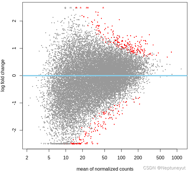
MA图对数据分布情况的可视化。该图将数据转换为M（对数比）和 A（平均值），然后绘制这些值来可视化两个样本中测量值之间的差异。

lfcshrink & MA plot

library(apeglm)  
resultsNames(dds_norm)  #看一下要shrink的维度;shrink数据更加紧凑,少了一项stat，但并未改变padj，但改变了foldchange
res_shrink <- lfcShrink(dds_norm, coef="condition_treat2_vs_treat1", type="apeglm") #最推荐apeglm算法;根据resultsNames(dds)的第5个维度，coef=5，也可直接""指定;apeglm不allow contrast，所以要指定coef
pdf("MAplot.pdf", width = 6, height = 6) 
plotMA(res_shrink, ylim=c(-10,10), alpha=0.1, main="MA plot: ")
dev.off()

After calling plotMA, one can use the function identify to interactively detect the row number of individual genes by clicking on the plot. One can then recover the gene identifiers by saving the resulting indices:

idx <- identify(res$baseMean, res$log2FoldChange)
rownames(res)[idx]

3.2 数据标准化

为了方便下游分析，DESeq2提供两种数据标准化方法:VST(variance stabilizing transformations)和rlog(regularized logarithm)。这两种方法都使用了log2缩放，并且已经进行了library size 或其他normalization factors的校正；这两种算法有着相同的特性，但大样本时（比如100个样本）VST运算更快，推荐使用VST。对于这两种算法的结果差异，本质上是y＝log2(n＋n0)公式中n0的估计值不一样。

提取两种算法标准化后的表达量：

#默认情况下blind=TRUE，但由于已经使用过DESeq()函数，无需重新估计dispersion值，因此这里blind=FALSE；
vsd <- vst(dds, blind=FALSE)
rld <- rlog(dds, blind=FALSE)
#对照：使用常规log2(n + 1)的标准化方法；
ntd <- normTransform(dds)
head(assay(vsd), 3)
head(assay(rld), 3)
head(assay(ntd), 3)

#导出标准化后的数据（可用于GSEA等下游分析）；

write.csv(as.data.frame(assay(vsd)),
file="count_transformation_VST.csv")
write.csv(as.data.frame(assay(rld)),
file="count_transformation_rlog.csv")
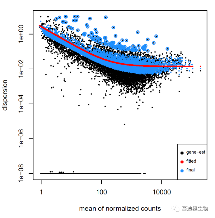
#绘制离散度散点图（Dispersion plot）；
#离群值未做收缩（shrunk）；
plotDispEsts(dds)

#对标准化后的数据进行可视化；

#BiocManager::install("vsn")
library("vsn")
library(ggplot2)
library(cowplot)
ntd1 <- meanSdPlot(assay(ntd))
vsd1 <- meanSdPlot(assay(vsd))
rld1 <- meanSdPlot(assay(rld))
p1 <- ntd1$gg+ggtitle("log2(n+1)")
p2 <- vsd1$gg+ggtitle("VST")
p3 <- rld1$gg+ggtitle("rlog")
plot_grid(p1, p2,p3,ncol = 3)

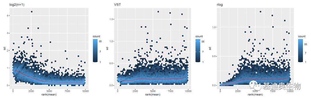
可见使用log2(n+1)标准化方法在低counts区域标准差较大，相反，rlog算法较大；而使用VST标准化后数据的标准差比较稳定；注意，虽然VST方法看起来效果最好，但图中的纵轴为方差的平方根（标准差），需要注意可能为由实验处理产生的真实方差。

3.3 常见的分析

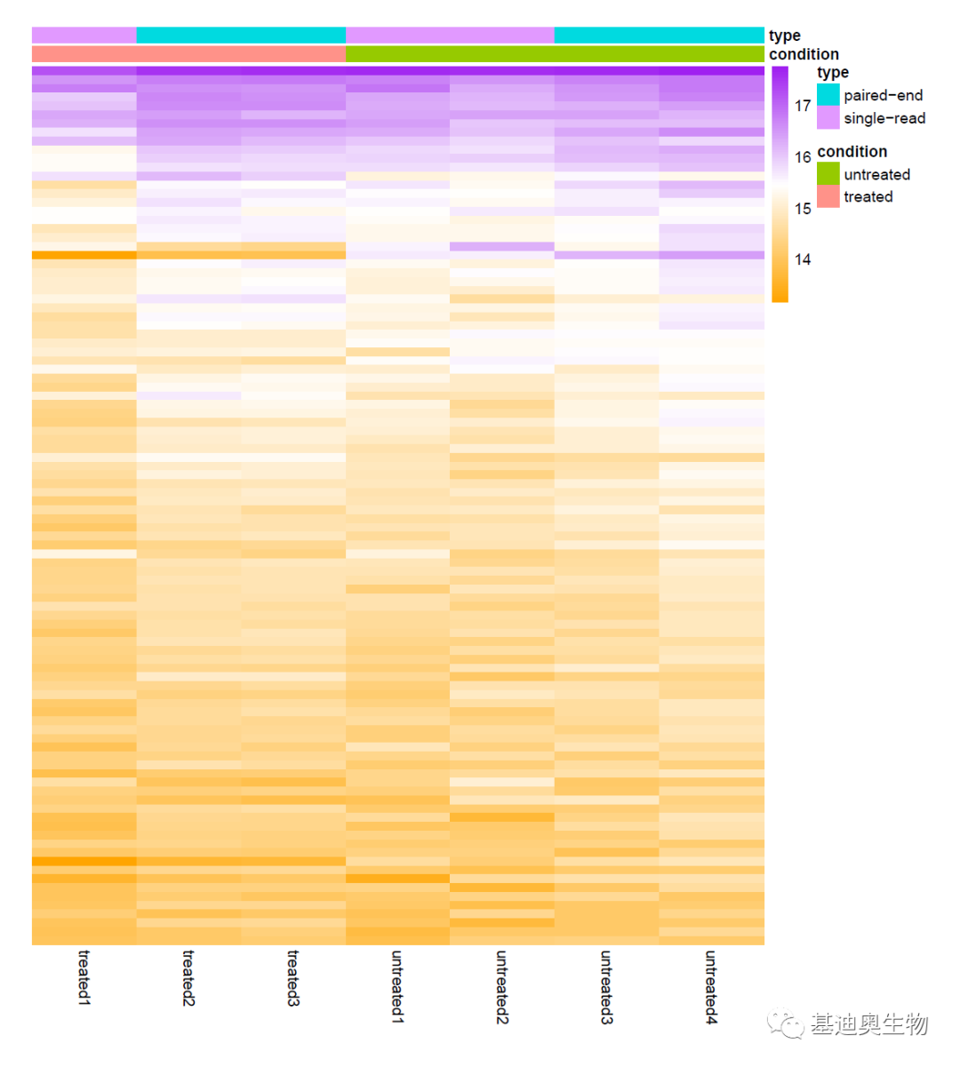
#使用标准化后平均表达量top100的基因绘制热图；

library("pheatmap")
select <- order(rowMeans(counts(dds,normalized=TRUE)),decreasing=TRUE)[1:70]

df <- as.data.frame(colData(dds)[,c('condition',"sampleid","type")])
mycolors = colorRampPalette(c("orange", "white","purple"))(70)

#vsd <- vst(dds, blind=FALSE) #大样本
rld <- rlog(dds, blind=FALSE)
pheatmap(assay(rld)[select,], cluster_rows=FALSE, show_rownames=TRUE,border_color=NA,color=mycolors,cluster_cols=FALSE, annotation_col=df)

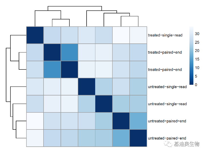
#绘制样本距离聚类热图；

#计算样本距离矩阵；
vsd<-rld
sampleDists <- dist(t(assay(vsd)))
#由向量转成矩阵；
sampleDistMatrix <- as.matrix(sampleDists)
rownames(sampleDistMatrix) <- paste(vsd$condition, vsd$type, sep="-")
colnames(sampleDistMatrix) <- NULL

#绘制聚类热图；
library("RColorBrewer")
colors <- colorRampPalette( rev(brewer.pal(9, "Blues")) )(255)
pheatmap(sampleDistMatrix,clustering_distance_rows=sampleDists,clustering_distance_cols=sampleDists,col=colors)

#PCA分析检查协变量和批次效应；

#生成pca作图数据；
pcaData <- plotPCA(vsd, intgroup=c("condition", "type"), returnData=TRUE)
#计算主成分的方差贡献率；
percentVar <- round(100 * attr(pcaData, "percentVar"))
library("ggplot2")
ggplot(pcaData, aes(PC1, PC2, color=condition, shape=type)) + geom_point(size=3) + xlab(paste0("PC1: ",percentVar[1],"% variance")) + ylab(paste0("PC2: ",percentVar[2],"% variance")) +coord_fixed()

#导出差异分析结果数据；

write.csv(as.data.frame(resOrdered),
file="condition_treated_results.csv")

#如果只导出差异基因，可使用subset函数； resSig <- subset(resOrdered, padj < 0.1) resSig write.csv(as.data.frame(resSig), file=“condition_treated_results_filtered.csv”)

3.4 多因素分析

我们最常见的是单因素差异分析，单因素实验设计比较简单，无需考虑不同因素之间的交互效应，比如研究年龄、身高与体重之间的关系，很显然体重与身高之间也有互作关系。类似常规多因素方差分析，DESeq2也支持多因素差异分析。

#例如本范例的数据包含两个因素：condition和type；
#查看样本信息（表型信息）；
colData(dds)
#创建（复制）一个新dds对象用于多因素差异分析；
ddsMF <- dds
levels(ddsMF$type)

#存在短线会出错（仅支持数字，点号，下划线），使用正则修改下名称；
#Tips: sub(pattern, replacement, x, ...)
levels(ddsMF$type) <- sub("-.*", "", levels(ddsMF$type))
levels(ddsMF$type)

#构建方程消除type（如批次效应）的影响（重点关心的因素放最后）；
design(ddsMF) <- formula(~ type + condition)
ddsMF <- DESeq(ddsMF)
resMF <- results(ddsMF)
head(resMF)

3.5 绘制带有基因名称的火山图

library(ggplot2)
library(ggrepel)
cut_off_stat = 0.05 #设置统计值阈值
cut_off_logFC = 1 #设置表达量阈值,可修改

diff_res <- as.data.frame(res)
diff_res$gene_id <- rownames(diff_res)
diff_res<-diff_res[, colnames(diff_res)[c(7,1:6)]]

diff_res[is.na(diff_res)] <- 0
diff_res$change = ifelse(diff_res$pvalue < cut_off_stat & abs(diff_res$log2FoldChange) >= cut_off_logFC, ifelse(diff_res$log2FoldChange> cut_off_logFC ,'Up','Down'), 'Stable')

diff_res$label = ifelse(diff_res$padj < cut_off_stat & abs(diff_res$log2FoldChange) >= 4, as.character(diff_res$gene_id),"")

pdf("./pre-post/volcanol_gene.pdf")

ggplot(diff_res,aes(x = log2FoldChange, y = -log10(padj), colour=change)) + geom_point(alpha=0.4, size=3.5) + scale_color_manual(values=c("#546de5", "#d2dae2","#ff4757"))+ geom_vline(xintercept=c(-1,1),lty=4,col="black",lwd=0.8) + geom_hline(yintercept = -log10(cut_off_stat),lty=4,col="black",lwd=0.8) + labs(x="log2(fold change)", y="-log10 (FDR)")+ theme_bw()+ theme(plot.title = element_text(hjust = 0.5), legend.position="right", legend.title = element_blank())+ geom_text_repel(data = diff_res, aes(x = diff_res$log2FoldChange, y = -log10(diff_res$padj), label = label), size = 3,box.padding = unit(0.8, "lines"), point.padding = unit(0.8, "lines"), show.legend = FALSE)

dev.off()

四、报错分析

4.1 报错

Error in checkSlotAssignment
> ## 6.提取结果，在treated和untreated组进行比较
> res <- results(dds, contrast = c("condition", "treated", "untreated")) 
Error in checkSlotAssignment(object, name, value) : 
  assignment of an object of class “DFrame” is not valid for slot ‘elementMetadata’ in an object of class “DESeqResults”; is(value, "DataTable_OR_NULL") is not TRUE

解决方法：

尝试使用.libPaths()查看DESeq2的位置，并找到删除，再重新运行安装命令，Update选择all.

参考资料

药企，独角兽，苏州。团队长期招人，感兴趣的都可以发邮件聊聊：tiehan@sina.cn

个人公众号，比较懒，很少更新，可以在上面提问题，如果回复不及时，可发邮件给我： tiehan@sina.cn