【4.5.3】验证曲线--绘制学习曲线

在我们在示例中看到的简单的一维问题中，很容易看出估计器是否存在偏差或方差。 然而，在高维空间中，模型可能变得非常难以可视化。 因此，使用验证曲线与学习曲线描述的工具通常很有帮助

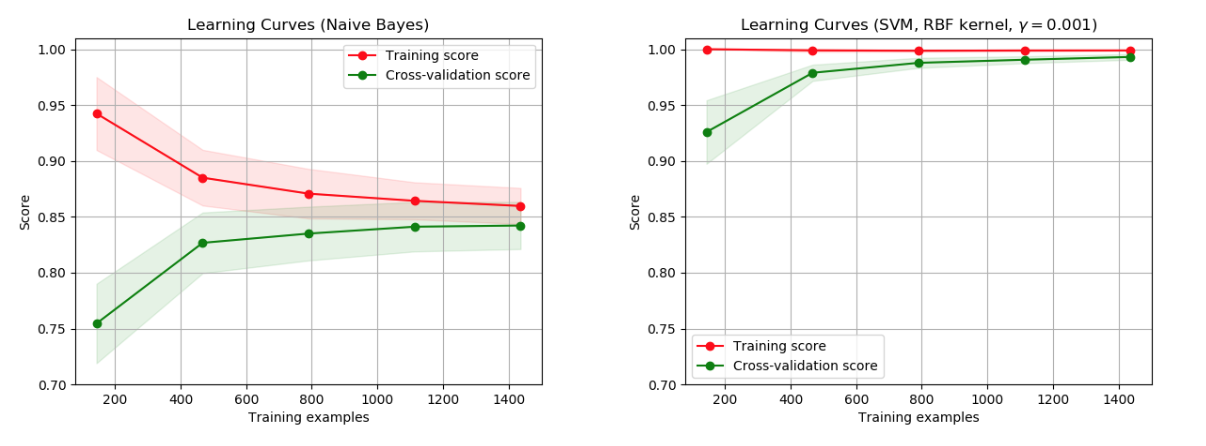
在左侧，显示了数字数据集的朴素贝叶斯分类器的学习曲线。 请注意，训练分数和交叉验证分数最终都不是很好。 然而，曲线的形状可以经常在更复杂的数据集中找到：训练分数在开始时非常高并且减少，并且交叉验证分数在开始时非常低并且增加。 在右侧，我们看到了带有RBF内核的SVM的学习曲线。 我们可以清楚地看到训练分数仍然在最大值附近，并且可以通过更多训练样本来增加验证分数。

学习曲线显示了针对不同数量的训练样本的估计器的验证和训练分数。 这是一个工具，可以找出我们从添加更多训练数据中获益的程度，以及估算器是否因方差误差或偏差误差而受到更多影响。 如果验证得分和训练得分都随着训练集的大小增加而收敛到太低的值，那么我们将不会从更多训练数据中获益。 在下图中你可以看到一个例子：朴素贝叶斯大致收敛到一个低分。

我们可能不得不使用当前估计器的估计器或参数化来学习更复杂的概念（即具有更低的偏差）。 如果训练分数远远大于最大训练样本数的验证分数，则添加更多训练样本很可能会增加泛化。 在下图中，您可以看到SVM可以从更多培训示例中受益。

代码：

print(__doc__)

import numpy as np
import matplotlib.pyplot as plt
from sklearn.naive_bayes import GaussianNB
from sklearn.svm import SVC
from sklearn.datasets import load_digits
from sklearn.model_selection import learning_curve
from sklearn.model_selection import ShuffleSplit


def plot_learning_curve(estimator, title, X, y, ylim=None, cv=None,
                        n_jobs=1, train_sizes=np.linspace(.1, 1.0, 5)):
    """
    Generate a simple plot of the test and training learning curve.

    Parameters
    ----------
    estimator : object type that implements the "fit" and "predict" methods
        An object of that type which is cloned for each validation.

    title : string
        Title for the chart.

    X : array-like, shape (n_samples, n_features)
        Training vector, where n_samples is the number of samples and
        n_features is the number of features.

    y : array-like, shape (n_samples) or (n_samples, n_features), optional
        Target relative to X for classification or regression;
        None for unsupervised learning.

    ylim : tuple, shape (ymin, ymax), optional
        Defines minimum and maximum yvalues plotted.

    cv : int, cross-validation generator or an iterable, optional
        Determines the cross-validation splitting strategy.
        Possible inputs for cv are:
          - None, to use the default 3-fold cross-validation,
          - integer, to specify the number of folds.
          - An object to be used as a cross-validation generator.
          - An iterable yielding train/test splits.

        For integer/None inputs, if ``y`` is binary or multiclass,
        :class:`StratifiedKFold` used. If the estimator is not a classifier
        or if ``y`` is neither binary nor multiclass, :class:`KFold` is used.

        Refer :ref:`User Guide <cross_validation>` for the various
        cross-validators that can be used here.

    n_jobs : integer, optional
        Number of jobs to run in parallel (default 1).
    """
    plt.figure()
    plt.title(title)
    if ylim is not None:
        plt.ylim(*ylim)
    plt.xlabel("Training examples")
    plt.ylabel("Score")
    train_sizes, train_scores, test_scores = learning_curve(
        estimator, X, y, cv=cv, n_jobs=n_jobs, train_sizes=train_sizes)
    train_scores_mean = np.mean(train_scores, axis=1)
    train_scores_std = np.std(train_scores, axis=1)
    test_scores_mean = np.mean(test_scores, axis=1)
    test_scores_std = np.std(test_scores, axis=1)
    plt.grid()

    plt.fill_between(train_sizes, train_scores_mean - train_scores_std,
                     train_scores_mean + train_scores_std, alpha=0.1,
                     color="r")
    plt.fill_between(train_sizes, test_scores_mean - test_scores_std,
                     test_scores_mean + test_scores_std, alpha=0.1, color="g")
    plt.plot(train_sizes, train_scores_mean, 'o-', color="r",
             label="Training score")
    plt.plot(train_sizes, test_scores_mean, 'o-', color="g",
             label="Cross-validation score")

    plt.legend(loc="best")
    return plt


digits = load_digits()
X, y = digits.data, digits.target


title = "Learning Curves (Naive Bayes)"
# Cross validation with 100 iterations to get smoother mean test and train
# score curves, each time with 20% data randomly selected as a validation set.
cv = ShuffleSplit(n_splits=100, test_size=0.2, random_state=0)

estimator = GaussianNB()
plot_learning_curve(estimator, title, X, y, ylim=(0.7, 1.01), cv=cv, n_jobs=4)

title = "Learning Curves (SVM, RBF kernel, $\gamma=0.001$)"
# SVC is more expensive so we do a lower number of CV iterations:
cv = ShuffleSplit(n_splits=10, test_size=0.2, random_state=0)
estimator = SVC(gamma=0.001)
plot_learning_curve(estimator, title, X, y, (0.7, 1.01), cv=cv, n_jobs=4)

plt.show()

learning_curve函数详解

我们可以使用函数learning_curve来生成绘制这样的学习曲线所需的值（已使用的样本数，训练集上的平均分数和验证集上的平均分数）：

from sklearn.model_selection import learning_curve
from sklearn.svm import SVC

train_sizes, train_scores, valid_scores = learning_curve(
    SVC(kernel='linear'), X, y, train_sizes=[50, 80, 110], cv=5)
train_sizes            

print train_scores           

print valid_scores           

结果

>>> train_scores           
array([[ 0.98...,  0.98 ,  0.98...,  0.98...,  0.98...],
       [ 0.98...,  1.   ,  0.98...,  0.98...,  0.98...],
       [ 0.98...,  1.   ,  0.98...,  0.98...,  0.99...]])
>>> valid_scores           
array([[ 1. ,  0.93...,  1. ,  1. ,  0.96...],
       [ 1. ,  0.96...,  1. ,  1. ,  0.96...],
       [ 1. ,  0.96...,  1. ,  1. ,  0.96...]])

参考资料

• http://scikit-learn.org/stable/auto_examples/model_selection/plot_learning_curve.html#sphx-glr-auto-examples-model-selection-plot-learning-curve-py
• http://scikit-learn.org/stable/modules/learning_curve.html