【9】例子--1--general--PCA与逻辑回归的搭配

Pipelining: chaining a PCA and a logistic regression PCA降维, logistic regression来作预测

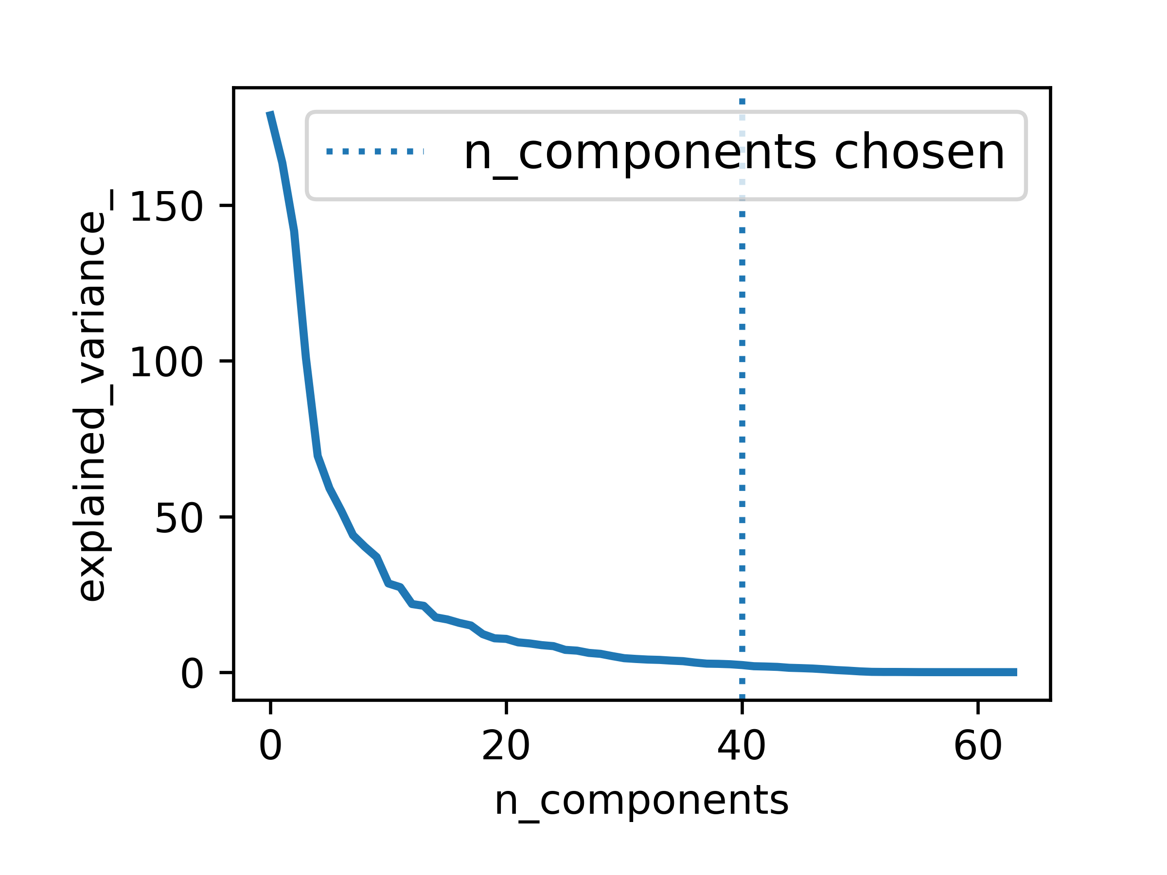
一、图：

二、代码：

#!/usr/bin/python
# -*- coding: utf-8 -*-

"""
=========================================================
Pipelining: chaining a PCA and a logistic regression
=========================================================

The PCA does an unsupervised dimensionality reduction, while the logistic
regression does the prediction.

We use a GridSearchCV to set the dimensionality of the PCA

"""
print(__doc__)


# Code source: Gaël Varoquaux
# Modified for documentation by Jaques Grobler
# License: BSD 3 clause


import numpy as np
import matplotlib.pyplot as plt

from sklearn import linear_model, decomposition, datasets
from sklearn.pipeline import Pipeline
from sklearn.model_selection import GridSearchCV

logistic = linear_model.LogisticRegression()

pca = decomposition.PCA()
pipe = Pipeline(steps=[('pca', pca), ('logistic', logistic)])

digits = datasets.load_digits()
X_digits = digits.data
y_digits = digits.target

###############################################################################
# Plot the PCA spectrum
pca.fit(X_digits)

plt.figure(1, figsize=(4, 3))
plt.clf()
plt.axes([.2, .2, .7, .7])
plt.plot(pca.explained_variance_, linewidth=2)
plt.axis('tight')
plt.xlabel('n_components')
plt.ylabel('explained_variance_')

###############################################################################
# Prediction

n_components = [20, 40, 64]
Cs = np.logspace(-4, 4, 3)

#Parameters of pipelines can be set using ‘__’ separated parameter names:

estimator = GridSearchCV(pipe,
						 dict(pca__n_components=n_components,
							  logistic__C=Cs))
estimator.fit(X_digits, y_digits)

plt.axvline(estimator.best_estimator_.named_steps['pca'].n_components,
			linestyle=':', label='n_components chosen')
plt.legend(prop=dict(size=12))
plt.savefig('chaining_PCA_and_logistic_regression',dpi=600)
plt.show()

三、撸代码：

1.digits = datasets.load_digits()

这个是手写数字数据集，包括1797个0-9的手写数字数据，每个数字由8*8 大小的矩阵构成，矩阵中值的范围是0-16，代表颜色的深度。

2.plt.clf()

清空当前的图片。我本来是要作图的，这个清空是几个意思呀？

Clear the current figure.

3.plt.axes([.2, .2, .7, .7])

在MATLAB中，axes是创建坐标轴对象，axis是修改坐标轴范围 axes(‘position’,[0.1 0.2 0.3 0.4]); % 创建一个坐标系。 %让起点是左边占到显示窗口的十分之一处，下边占到十分之二处。 %，宽占十分之三，高占十分之四。一个小框就出来了。

4.np.logspace(-4,4,3)

1.00000000e-04 1.00000000e+00 1.00000000e+04] 个数为3，起始e-4，终止为e4的等比数列

5.axvline

matplotlib.pyplot.axvline(x=0, ymin=0, ymax=1, hold=None, **kwargs) 在图中话一条竖直（vertical）的线

6.PCAH和逻辑回归算法略

参考资料：

http://blog.csdn.net/bea_tree/article/details/51089035

http://scikit-learn.org/stable/auto_examples/plot_digits_pipe.html#sphx-glr-auto-examples-plot-digits-pipe-py